−Table of Contents
Radially Averaged Autocorrelation
An ImageJ macro that calculates the radial average of the autocorrelation of a (binary) image.
For the autocorrelation (radial distribution) of particle centers, see the Radial Distribution Function macro.
Description
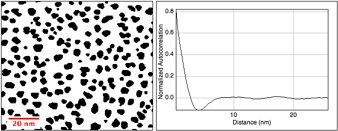
The macro calculates the autocorrelation (also known as pair correlation or two-point correlation) of the pixels of an image as a function of distance. Although it uses the Fourier transform, it does not suffer from artifacts caused by the 'periodic' nature of the FFT. Also, it corrects for the finite image size, assuming that the image shows a random part of a much larger area having the same autocorrelation.
The autocorrelation is scaled in such a way that an output of zero means 'no correlation' and one means 'perfect correlation'. The lower limit of -1 would mean 'perfect anticorrelation' at a given distance. Thus, at a distance of r = 0, the value is always one (this value is not included in the output).
The autocorrelation gives information about the typical feature size in an image. Bear in mind that this information combines both the particles and the holes in between them (when scaled, the autocorrelation is the same for an image and its inverse, with particles and holes exchanged). The initial slope, first zero and first minimum include information on particle and hole sizes; the first side maximum of the autocorrelation gives the typical distance between two particles or holes.
Notes for using in porosity analysis
In porosity analysis (e.g. of rocks), the correlation function S (also named Rz) is often defined without a diffferent normalization, such that S(0) is equal to the pore fraction Φ, and absence of correlation is denoted by a value of S = Φ2. See, e.g., J.G. Berryman, S.C. Blair, J. Appl. Phys. 60, 1930 (1986). You can use a simple linear transformation to get these values from the output A of the macro:
S(r) = Φ2 + A (Φ - Φ2)
Note that the low values of the autocorrelation at large distances r [around the second zero of A(r) and beyond] are usually not very trustworthy unless you average over a large number of images. When calculating scattering functions (e.g. for small-angle neutron scattering) from the autocorrelation, these values can have a large effect on the result, because they get multiplied with r2 in the integral. See, e.g., Equation (1) in Radlinski et al., J. Colloid Interf. Sci. 274, 607 (2004) for the conversion from the correlation function (here named Rz) to the scattering intensity.
The macro
Limitations: The macro assumes square pixels (pixel aspect ratio = 1).
The macro needs the Radial_Profile plugin (May 2009 version!)
// ImageJ macro to calculate the Radially Averaged Autocorrelation Function,
// Corrected for finite size effects
// The output is normalized to a value of 1 at zero radius
// and corrected for effects of the finite image size.
// (No need to extend the image size for avoiding edge effects)
//
// Use with a binary input image.
// Needs the last (2008-05-14) Version of the "Radial Profile Plot" plugin,
// http://rsb.info.nih.gov/ij/plugins/radial-profile.html
//
// Version: 2011-Sep-27 Michael Schmid: fixes bug when processing stack (normalization was wrong)
// Version: 2015-Feb-17 Michael Schmid: added missing Plot.show(); at the end
//
requires("1.42p");
doStack=false;
if (nSlices()>1) doStack = getBoolean("Get RDF from full stack?");
setBatchMode(true);
firstSlice=getSliceNumber();
lastSlice=getSliceNumber();
if (doStack) {
  firstSlice=1;
  lastSlice=nSlices();
}
width=getWidth;
height=getHeight;
getPixelSize(unit, pixelWidth, pixelHeight);
run("Select None");
//maxRadius may be modified, should not be larger than 0.3*minOf(width, height);
maxRadius=0.3*minOf(width, height);
minFFTsize=1.3*maxOf(width, height);
title=getTitle();
size=4;
while(size<minFFTsize) size*=2;
for (slice=firstSlice; slice<=lastSlice; slice++) {
  if (doStack) setSlice(slice);
  //make autocorrelation of particle image
  tempTitle="temp-"+random();
  run("Duplicate...", "title="+tempTitle);
  tempID=getImageID();
  getRawStatistics(nPixels, mean);
  run("Canvas Size...", "width="+ size+" height="+ size+" position=Center zero");
  makeRectangle(floor((size-width)/2), floor((size-height)/2), width, height);
  run("Make Inverse");
  run("Set...", "value="+mean);
  run("Select None");
  getRawStatistics(nPixels, mean);
  run("FD Math...", "image1=["+tempTitle+"] operation=Correlate image2=["+tempTitle+"] result=AutoCorrelation do");
  psID=getImageID();
  run("Subtract...", "value="+(nPixels*mean*mean));
  selectImage(tempID);
  close();

  //make autocorrelation reference to correct finite image size effects
  newImage("frame", "8-bit White", width, height, 1);
  run("Set...", "value=255");
  tempID=getImageID();
  rename(tempTitle);
  run("Canvas Size...", "width="+ size+" height="+ size+" position=Center zero");
  run("FD Math...", "image1=["+tempTitle+"] operation=Correlate image2=["+tempTitle+"] result=AutoCorrReference do");
  refID=getImageID();
  imageCalculator("Divide", psID,refID);
  selectImage(refID);
  close();
  selectImage(tempID);
  close();

  //prepare normalized power spectrum for radial averaging
  selectImage(psID);
//  makeRectangle(size/2, size/2, 1, 1);
//  run("Set...", "value=0");
//  run("Select None");
  circleSize=2*floor(maxRadius)+1;
//  run("Specify...", "width="+circleSize+" height="+circleSize+" x="+(size/2+0.5)+" y="+(size/2+0.5)+" oval centered");
//  getRawStatistics(nPixels, mean);
//  run("Select None");
//  run("Divide...", "value="+mean);
  norm = getPixel(size/2, size/2);
  run("Divide...", "value="+norm);
  run("Specify...", "width="+circleSize+" height="+circleSize+" x="+(size/2+0.5)+" y="+(size/2+0.5)+" oval centered");
  run("Radial Profile", "x="+(size/2+0.5)+" y="+(size/2+0.5)+" radius="+floor(maxRadius)-1);
  plotID=getImageID();
  Plot.getValues(x, y);
  if (slice==firstSlice) ySum = newArray(y.length);
  for (i=0; i<y.length; i++)
    ySum[i]+=y[i]/(lastSlice-firstSlice+1);
  selectImage(plotID);
  close();
  selectImage(psID);
  close();
}
setBatchMode("exit and display");
if (pixelWidth==pixelHeight) {
  for (i=0; i<x.length; i++)
    x[i] *= pixelWidth;
} else
  unit = "pixels";
if (doStack) title = title + " (stack)";
Plot.create("Autocorrelation of "+title, "Distance ("+unit+")", "Normalized Autocorrelation", x, ySum);
Plot.show();
If you want the data in the plot as a list, add the following lines at the end of the macro:
run("Clear Results");
Plot.getValues(xpoints, ypoints);
for (i=0; i<xpoints.length; i++) {
  setResult("R", i, xpoints[i]);
  setResult("AC", i, ypoints[i]);
}
